Section 2 · Lesson 4
Engineer features and target encodings
Build the features that lifted macro F1 from 0.730 to 0.758, and learn why out-of-fold target encoding works.
- Why the final notebook turns
operator_refinto counts instead of using it as a category. - Which features gave the biggest gains, with the experiment numbers.
- How smoothed target encoding works, and why out-of-fold encoding prevents leakage.
- What residual encoding adds, and why those features rank first in importance.
How the project searched for features
Feature work ran as three parallel experiment tracks (experiments/fe, te, and models). Every run used the same 20% holdout, the first fold of a five-fold stratified split with seed 42, so the scores are comparable. Rerunning the baseline with different thread counts and seeds moved the score by about 0.002, so treat smaller differences as noise.
Basic features: nothing from the label
The notebook's basic_features() function builds features without using the target. It processes train and test together so both get the same columns and category levels. The following excerpt shows the identifier and facility handling:
for c in ["operator_ref", "zone", "borough"]:
    df[c] = raw[c].map(raw[c].value_counts())     # ID -> listing count
df["n_facilities"] = df["facilities"].str.count("FCL-")

codes = raw["facilities"].fillna("[]").map(json.loads).explode().dropna()
fac = pd.crosstab(codes.index, codes).reindex(raw.index, fill_value=0).clip(upper=1)
fac.columns = ["f_" + c[4:] for c in fac.columns]  # one 0/1 column per code
Each block earns its place:
- Flags and dates.
tandfbecome 1 and 0. Dates become day counts since 2000-01-01. - IDs as counts.
operator_ref(about 42,000 values),zone, andboroughbecome the number of listings that share the value. As raw LightGBM categories, they overfit badly, especiallyoperator_ref, and 34% of test listings have an operator that never appears in train. - Facilities. The list becomes 145 binary columns plus a count. The notebook processes train and test together, which is why it finds 145 codes where the training data alone has 144. This block gave the largest gain of any non-target feature.
- Geography. Sums, differences, and rotations of the coordinates (15, 30, and 60 degrees) let trees draw diagonal boundaries. Distances to the metro and zone centers, and a 100-cluster k-means label with the distance to its center, are also added.
The feature experiments
The following holdout scores come from experiments/fe/results.tsv. The model is a LightGBM multiclass model. "Freq only" means the ID column is replaced by its listing count.
| Feature set | Holdout macro F1 | Change from base |
|---|---|---|
| Base (raw columns, IDs as categories) | 0.7303 | 0 |
| Base + all facility flags | 0.7344 | +0.0041 |
Base + operator_ref as count only | 0.7336 | +0.0033 |
| Base + operator and zone as counts only | 0.7377 | +0.0074 |
| ... + facility flags | 0.7476 | +0.0173 |
| ... + geography | 0.7503 | +0.0200 |
| Facility TF-IDF with SVD, ratio features, date differences, group aggregates | within noise | about 0 |
Target encoding
A target encoding replaces a category with a statistic of the label for that category. Here the statistic is the smoothed share of each tier among the listings in the group. For group \(g\) with \(n_g\) listings, \(n_{g,k}\) of which are tier \(k\), and overall tier share \(\pi_k\):
$$\hat p_{g,k} = \frac{n_{g,k} + m\,\pi_k}{n_g + m}$$The smoothing weight \(m\) is 20 in the notebook. A group with few listings gets pulled toward the overall class mix, and a large group keeps its own mix. Without smoothing, a group with a single listing would claim 100% for its tier.
The notebook encodes 15 groups, such as operator, zone, operator and zone together, and near-duplicate listings that share operator, zone, space class, and seat count. For each group it creates four tier shares (_p1 to _p4), the mean tier, and the log group size.
Why out-of-fold encoding matters
If you compute the encoding of a training row from a group that includes that row, the row's own label leaks into its feature. The model learns to trust the feature, which looks perfect on training rows and fails on new ones. The fix is out-of-fold (OOF) encoding: split the training rows into five folds, and compute each fold's encodings from the other four. For test rows, use all of train.
T_train = pd.concat([target_features(fit, val).set_index(val)
                     for fit, val in folds]).sort_index()
T_test = target_features(np.arange(len(train)),
                         np.arange(len(train), len(both)))
Here fit holds the other four folds and val holds the rows being encoded.
Target-encoding playground
Pick a real operator group from the training data, or type your own tier counts. Move the smoothing slider, then compare what a row sees when its own label is included (in-sample) and when it's left out. The out-of-fold view here uses a leave-one-out approximation. The notebook uses five folds.
Try the single-listing groups at the top of the list with m set to 0. The in-sample encoding matches the row's tier 100% of the time, which looks like skill but is only the row's own label coming back. Raise m and that false confidence shrinks toward the prior.
A leakage experiment you can reproduce
The course script build/03_leakage_experiment.py isolates the effect. It trains a small LightGBM on only the operator target encoding, on fold 0 of the project's split. This experiment is not part of the original project, and the numbers are specific to this setup.
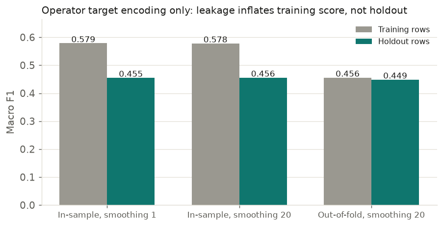
The lesson is that the training score is no longer honest with in-sample encoding. The holdout scores differ little in this single-feature setup, because the model has nothing else to trust. In the full 350-feature model, the same flaw would let the model over-rely on the encodings.
Residual encoding: the strongest feature
Some operators charge a premium. Others only rent large spaces. A plain target encoding can't tell the two apart. Residual encoding separates them:
- Estimate the typical tier for each combination of
access_typeandmax_seats. - For operator, zone, location, and space-class groups, average how far each listing's tier sits above or below that baseline.
- Add the group's average residual back to the baseline for the row's own seat and access combination, to get
res_*_pred.
The notebook also adds geographic neighbors: the tier mix of the listings at the 1, 5, 20, and 50 nearest distinct coordinates.
Target-feature experiments
The following scores come from experiments/te/results.tsv, with the same holdout:
| Setup | Holdout macro F1 |
|---|---|
| Base (raw IDs as categories) | 0.7284 |
| Basic target encodings, raw IDs still included | 0.7270 |
| Basic target encodings, raw IDs dropped | 0.7420 |
| + residual encodings | 0.7461 |
| + residual encodings and geographic neighbors | 0.7475 |
| All encodings, residuals, and neighbors, raw IDs dropped | 0.7505 |
Two results stand out. First, adding target encodings while the raw IDs stay in the model doesn't help, because LightGBM still overfits the IDs. Dropping them is what unlocks the gain. Second, each new family adds a little more.
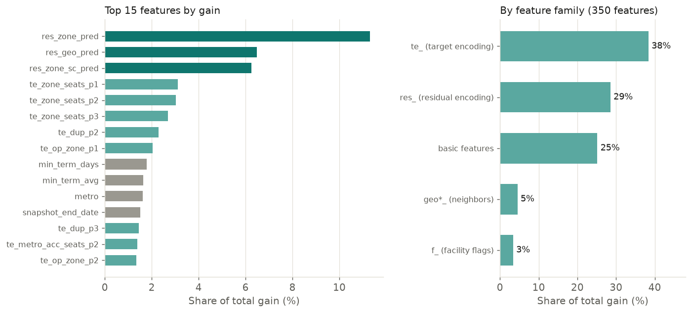
build/02_importance.py with the notebook's own feature code. Residual encodings take the top three places.You add target encodings for operator_ref, but the model still uses the raw operator_ref as a categorical column. What did the experiments find?
- The score didn't improve (0.727 against a 0.728 base), because the model kept overfitting the raw IDs.
- The score jumped by 0.02.
- The score dropped to 0.
Dropping the raw high-cardinality IDs (0.742) was necessary for the target encodings to help.
For test rows, which listings does the notebook use to compute target encodings?
- Only the test rows themselves.
- The four folds not used for that row, as in training.
- All rows in train, because test labels are unknown and no row's label is at risk of leaking.
Test rows never have their own label in the data. Using all of train gives them the best encoding, and the training rows' OOF encodings imitate that situation.