Section 2 · Lesson 5
Compare models, from baseline to boosting
Trace the path from default LightGBM to categorical regularization, ordinal models, and CatBoost.
- How gradient boosting builds a model one small tree at a time.
- Why regularizing categorical splits gave the largest single-model gain.
- How an ordinal model uses the tier order, and what
cumulative_to_classes()does. - Why CatBoost won on single-model score but missed the final notebook.
Gradient boosting in one paragraph
A boosted model starts with a constant prediction. Then it repeats the following loop: measure the residuals (how far each prediction is from the truth), fit a small decision tree to those residuals, and add a fraction of that tree, set by the learning rate, to the prediction. Each round corrects what the earlier trees missed. The following demo runs the loop on a one-dimensional curve.
Boosting stepper on 1-D data
Click Add tree to fit one tree to the residuals. The blue line is the model, the gray lines are the residuals, and the error falls with each round. Try depth 1 (a single split) against depth 3, and a small learning rate against a large one.
The following video runs the same idea on real data. It trains LightGBM on only geo_lat and geo_lon for the largest-spread metro, MTR-01, and shows the decision regions after each round. Holdout macro F1 climbs from 0.152 after one round to 0.421 after 300 rounds. With two features only, this is far below the full model, but the mechanism is the same.
build/04_videos.py) made it from train.csv.The model ladder
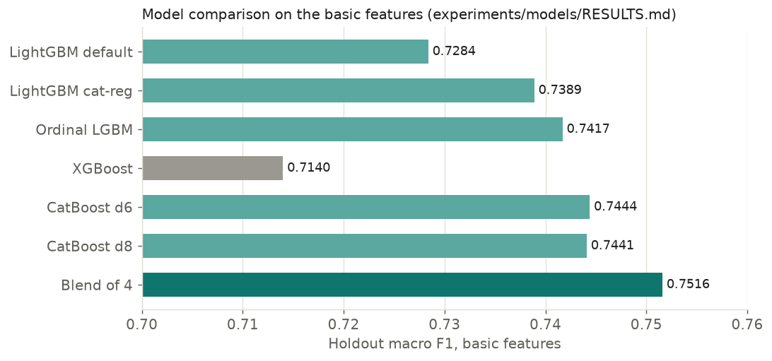
The model experiments (experiments/models/RESULTS.md) use the basic features and the same holdout of 55,950 rows. The first row is the baseline.
| Experiment | Holdout macro F1 | Change | Log loss |
|---|---|---|---|
| LightGBM, default categoricals | 0.7284 | 0 | 0.6284 |
LightGBM, num_leaves 63 | 0.7269 | -0.0014 | 0.6347 |
LightGBM, num_leaves 255 | 0.7302 | +0.0019 | 0.6237 |
LightGBM, regularized categoricals (cat_smooth 200, cat_l2 200, min_data_per_group 1000, max_cat_threshold 16) | 0.7389 | +0.0105 | 0.6027 |
Same, but operator_ref dropped | 0.7356 | +0.0072 | 0.6080 |
| LGBM regression, rounded | 0.7325 | +0.0041 | n/a |
| Ordinal LightGBM (three binary models) | 0.7417 | +0.0133 | 0.6092 |
| XGBoost, native categoricals | 0.7140 | -0.0144 | 0.6856 |
| CatBoost, depth 8 | 0.7441 | +0.0157 | 0.5885 |
| CatBoost, depth 6 | 0.7444 | +0.0160 | 0.5890 |
Regularize the categorical splits
The biggest single-model gain (+0.0105 and a log loss drop from 0.628 to 0.603) came from changing four LightGBM parameters that control how it splits categorical columns. With about 42,000 operator levels, default categorical splitting memorizes operators. Dropping operator_ref or using integer codes was worse than regularizing it, which shows that the column carries signal. After this change, the sweeps of num_leaves, min_child_samples, feature_fraction, and lambda_l2 were all within noise.
The final notebook solved the same problem differently. It replaced the IDs with counts and target encodings (Lesson 4), which worked better than regularizing them.
Use the order of the tiers
An ordinal model respects the order 1 < 2 < 3 < 4. Instead of one four-class model, it trains three binary models, one each for P(tier > 1), P(tier > 2), and P(tier > 3). The notebook's cumulative_to_classes() turns them into class probabilities:
def cumulative_to_classes(p_above):
    p_above = np.minimum.accumulate(p_above, axis=1)   # keep P(>1) >= P(>2) >= P(>3)
    edges = np.column_stack([np.ones(len(p_above)), p_above, np.zeros(len(p_above))])
    return np.clip(edges[:, :-1] - edges[:, 1:], 1e-6, 1)
The probability of tier \(k\) is P(tier > \(k-1\)) minus P(tier > \(k\)). Three independent models can disagree and produce a negative result, so np.minimum.accumulate forces the sequence to be non-increasing.
Ordinal decoder
Set the three cumulative probabilities that the binary models predict for one listing. The decoder shows the four class probabilities. Make the sliders disagree (for example, P(>2) above P(>1)) to see the monotone fix.
The ordinal model beat multiclass LightGBM by about 0.003 macro F1 and trained in about 100 seconds. Its bigger value is diversity: it makes different errors from multiclass models, so it adds more to a blend than another multiclass model does.
Why does cumulative_to_classes() call np.minimum.accumulate?
- To make the probabilities sum to 2.
- To keep P(>1) ≥ P(>2) ≥ P(>3), so no class probability comes out negative.
- To speed up prediction.
The three binary models are trained independently, so their outputs can cross. The accumulate step removes the crossings.
CatBoost: strongest alone, left out of the notebook
CatBoost with native categoricals was the strongest single model (about 0.744 and log loss 0.589), but one fit took 33-37 minutes at four threads. On the full feature set it reached 0.753 and added only +0.0003 to the blend, at about 12 minutes per fold. The final notebook leaves it out to stay short and fast.
Dead ends worth knowing
- XGBoost with native categoricals overfit through
operator_ref(best iteration 130, macro F1 0.714) and was slow. It would needoperator_refhandled differently. - Regression with tuned cut points scored 0.734, below multiclass with argmax.
- Balanced class weights during training were within noise.
After categorical regularization, you try num_leaves 255 and get 0.7383 against 0.7389. What do you conclude?
- 255 leaves is clearly worse, so you must never raise it.
- 255 leaves is clearly better, so you should always raise it.
- The changes are close to the run-to-run noise (about 0.002), so don't over-interpret them.
The 0.0006 difference is well under the noise. The notebook picks 127 leaves, the value in its parameter set.