Section 2 · Lesson 3
Preprocess without leaking
Turn raw columns into clean numbers, and fit every learned step on training data only.
- How the project cleaned duplicates, invalid values, and missing values.
- Why heavy-tailed counts get clipped and log-transformed for linear models, but not for trees.
- The rule that keeps validation scores honest: fit on training data only.
- How preprocessing lifted a logistic regression from 0.358 to 0.682 macro F1.
Two pipelines for two jobs
The project has two preprocessing designs, and the difference teaches you something:
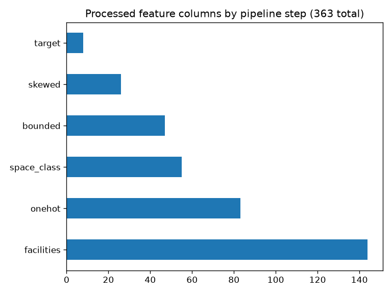
- The Milestone 2 pipeline builds a clean, scaled, fully numeric matrix of 363 columns for a logistic regression baseline.
- The final notebook feeds LightGBM, which doesn't need scaling or one-hot encoding. It uses a lighter set of steps and the target features from Lesson 4.
Both follow the same safety rule, covered later in this lesson.
Clean the data
Milestone 2 handled each data-quality issue with a stated reason:
| Issue | Rows | Action | Reason |
|---|---|---|---|
| Exact duplicates | 1,116 | Drop from train (leaves 278,630 rows) | Copies in both a training fold and a validation fold inflate the score. |
| Conflicting duplicates | 43 groups | Keep | You can't tell which label is right. |
Invalid max_term_* | 62 | Cap at 1,125 days | The rest of each row is valid. |
| Scores with zero reviews | 4 | Set scores to missing | Matches the 54,000 other unreviewed listings. |
The project doesn't drop duplicates from the test set, because every test listing needs a prediction.
Fill missing values
The method follows the reason for the gap (Lesson 2):
boroughgets a separatenonelevel.- Review fields,
zones,utility_rooms, andworkstationsget the median plus a missing indicator, so the model can still see that the value was absent. operator_refbecomesunknownwhen the whole operator profile is missing.
Dropping rows would lose 20-77% of the data. Mean imputation gets pulled by the long right tails. KNN and iterative imputation are slow on 280,000 rows and add little for tree models.
Tame heavy tails
Count columns such as review_count have long right tails. For the linear baseline, the pipeline winsorizes at the 0.5th and 99.5th training percentiles, applies log1p, and then scales. The skew of review_count falls from 5.36 to 0.08. The clip bounds are learned in fit, so a custom transformer stores them:
class Clipper(BaseEstimator, TransformerMixin):
    def __init__(self, low=0.005, high=0.995):
        self.low, self.high = low, high
    def fit(self, X, y=None):
        self.lo_ = np.nanquantile(X, self.low, axis=0)
        self.hi_ = np.nanquantile(X, self.high, axis=0)
        return self
    def transform(self, X):
        return np.clip(X, self.lo_, self.hi_)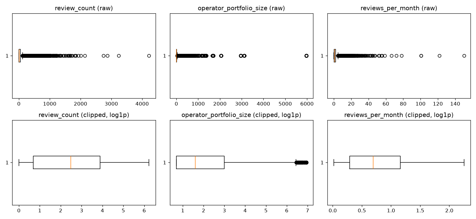
log1p (Milestone 2, Figure Q4.1).Clip and log-transform a skewed count
The data is a synthetic log-normal sample of 4,000 values, standing in for a column such as review_count. Lower the clip percentile and switch on log1p, and watch the skewness drop.
Trees don't care. Gradient-boosted trees split on the order of values, so clipping, logs, and scaling change little for them. The project applies these steps in Milestone 2 because the baseline is a logistic regression, which is sensitive to scale. The final LightGBM notebook skips them.
Encode categories by their cardinality
Milestone 2 chose an encoding for each column based on its number of levels:
- One-hot for low-cardinality columns:
operator_class,access_type,compliance_status,metro, andborough. These add 83 columns, withhandle_unknown="ignore". - One-hot with rare levels grouped for
space_class: 131 levels, 77 of them with fewer than 30 rows, collapse to 55 columns withmin_frequency=30. - Target encoding for
operator_ref(41,903 values) andzone(1,380 values). One-hot encoding these would add more than 43,000 sparse columns. - Multi-hot for
facilities, and durations instead of raw dates.
Fit on training data only
Data leakage means information from outside the training data influences the model or its validation score. The most common cause is fitting a learned step, such as an imputer's median, a scaler's mean, or an encoder's category means, on data that includes the validation fold or the test set. The score looks better than reality, and the gap appears only on new data.
The project follows these rules:
- Fit every learned step with
fiton training data only. Validation folds and the test set only go throughtransform. - Put the whole pipeline inside
cross_val_score, so it refits on each training fold. - Use cross-fitting for target encoding, so a row never sees its own label (Lesson 4).
- In Milestone 2, drop exact duplicates before you split, so copies can't straddle a train and validation fold.
You compute the median of review_count from train and validation together, then fill the gaps in both. What went wrong?
- Nothing. The median is only a summary.
- The validation fold influenced a learned step, so the validation score is slightly optimistic.
- The median should have been the mean.
Any statistic computed with validation rows leaks a little information about them. The effect is small for a median, but the habit matters, and it grows large for learned encodings.
Does preprocessing matter? A logistic regression test
Milestone 2 tested the effect on a logistic regression, with 5-fold stratified cross-validation and macro F1. The minimal setup used only the numeric columns with median filling. The preprocessed setup used the full pipeline, refit inside each fold.
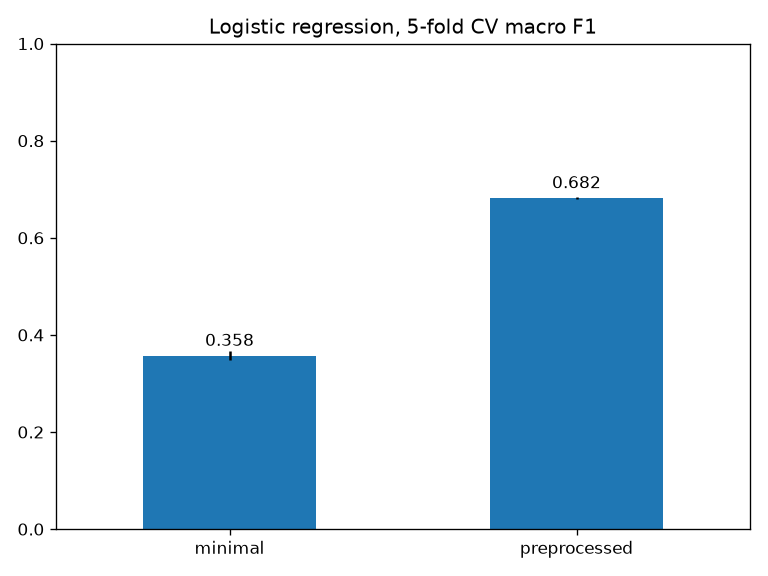
The minimal model scores far lower partly because unscaled columns such as max_term_days, in the hundreds of millions, make the optimization badly conditioned, so 300 iterations aren't enough. It also lacks every categorical, facility, and operator signal. For context, the final LightGBM notebook reaches about 0.758.
Why does the final LightGBM notebook skip scaling and one-hot encoding?
- LightGBM can't read scaled data.
- Scaling always hurts accuracy.
- Trees split on the order of values, so scale doesn't matter, and LightGBM handles categories natively.
Scale matters for linear and distance-based models. The notebook instead spends its effort on features that tell the trees something new.