Section 1 · Lesson 2
Exploring the data
Before you train anything, count what you have. The class balance, the mask sizes, and the empty images decide almost every later choice.
- How rare each defect is, and how often defects co-occur.
- How small the masks are, and why that matters for filtering.
- Why the project splits the data by label combination.
Class balance
Almost half of the images, 5,516 of 11,393, have no defect at all. Among the rest, defect_c is the most common (4,100 images) and defect_b is rare (313 images). Counting pairs (one image and one defect type) makes the imbalance sharper: 38,371 of the 45,572 pairs are empty, which is 84.2%.
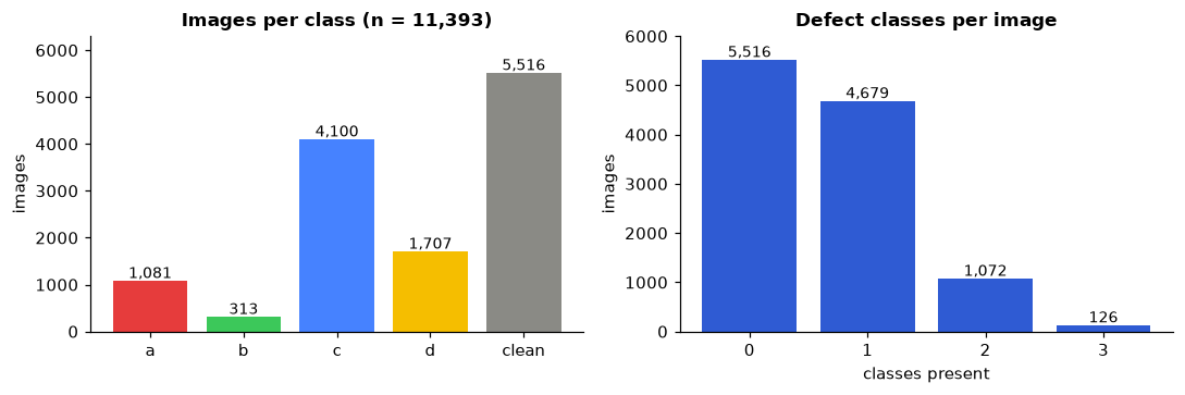
Images can carry several defects. 4,679 images have one class, 1,072 have two, and 126 have three. The milestone analysis (milestone1/analysis.py) also checks the pixels: the masks of different classes never overlap, so each pixel belongs to at most one class.
Dataset explorer
Switch the view to see the label statistics computed from train.csv.
Label combinations
The labels form 15 combinations, such as defect_c alone, defect_c+defect_d, or clean. The rarest, defect_a+defect_b+defect_c, has only 8 images.
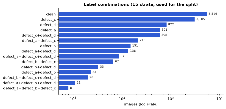
The project splits the data into 80% training and 20% holdout, and stratifies on this combination string rather than on one class. That keeps rare combinations in both parts. This function is in src/common.py:
def combo_string(row):
    present = [c for c in CLASSES if isinstance(row[c], str) and row[c].strip()]
    return "+".join(present) if present else "clean"

def stratified_split(wide, val_frac=0.2, seed=42):
    combos = wide.apply(combo_string, axis=1)
    counts = combos.map(combos.value_counts())
    single = counts < 2          # a stratum with one image can't be split
    tr, va = train_test_split(wide[~single], test_size=val_frac,
                              stratify=combos[~single], random_state=seed)
    tr = pd.concat([tr, wide[single]])
    return tr.reset_index(drop=True), va.reset_index(drop=True)
The result is 9,114 training images and 2,279 holdout images. The holdout contains 63 images with defect_b, so scores for that class are noisy. Keep this in mind when you read the results later.
Where and how big
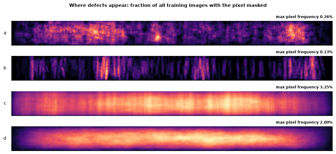
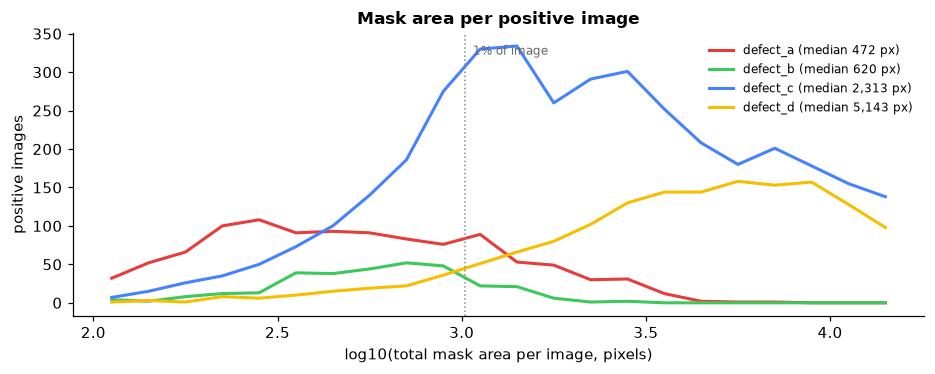
The next step splits each mask into connected components (separate blobs). The results come from milestone1/analysis.py, question 10:
| Class | Components | Smallest (px) | Median (px) |
|---|
What a minimum-area filter deletes
Post-processing often removes small blobs. Choose a cutoff N to see what share of each class's true mask pixels sits in components smaller than N. Those pixels are lost if the filter removes them.
A cutoff of 200 pixels removes 15.2% of the defect_a mask but under 0.4% of defect_c and defect_d. A single global cutoff would hurt defect_a and defect_b most. This is why lesson 6 tunes a separate cutoff for each class.
Do defects look different from the background?
The milestone analysis computes Cohen's d between the gray levels of defect pixels and the background pixels of the same image. A value near 0 means the defect has the same brightness as its surroundings.
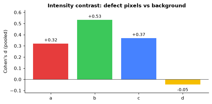
defect_d is about 0, so only texture, not brightness, identifies it.defect_b has the largest contrast (0.53), and defect_d has almost none (-0.05). A model can't separate defect_d by brightness alone. It has to learn the texture, which is one reason the project uses a convolutional network instead of a simple threshold.
Takeaway. The data is mostly empty, one class is rare, and masks are small. Accuracy-style metrics would reward predicting nothing. The next lesson shows how the competition score handles this.
Why does the split stratify on the combination string instead of on each class separately?
- It makes the training set larger.
- It keeps every label combination, including rare ones, in both training and holdout.
- It removes images with several defects.
Stratifying on the full combination preserves the joint label pattern, so rare combinations with defect_b appear in both parts. The holdout gets 63 defect_b images.
A minimum-area filter of 200 pixels removes which share of the true defect_a mask pixels?
- About 15%
- About 1%
- About 50%
The analysis finds that 15.22% of defect_a mask pixels sit in components under 200 pixels. At 500 pixels the loss rises to 50.9%.