Section 1 · Lesson 8
Lessons learned and recap
The score climbed from 0.30 to 0.6486 because of decisions about the metric and the data, more than because of a fancier network.
- Which choices moved the score, with the numbers.
- What the project can't claim, and how to extend it.
- A recap quiz covering the whole section.
The path to 0.6486
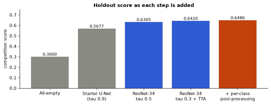
| Step | Score | Source |
|---|---|---|
| Predict nothing | 0.3000 | milestone1/answers.json, question 9 |
| Milestone 1 starter model, tau 0.9 | 0.5677 | threshold_sweep.csv |
| ResNet-34 U-Net with TTA, tau 0.5 | 0.6305 | runs/r34_baseline/eval.json |
| Same, tau 0.3 | 0.6420 | eval.json |
| Same, per-class post-processing (2-fold CV) | 0.6486 | eval.json |
What worked
- Read the metric before modelling. The all-empty baseline scores 0.30, and naive Dice rewards silence. Knowing that a missed defect costs about 37 times more than a false alarm pointed the project toward low thresholds from the start.
- Split on label combinations. Stratifying on the 15-way combination string kept rare classes in the holdout (63
defect_bimages). - Keep the native 128 × 800 shape. No resizing means no aspect distortion, and both dimensions divide by 32 for the encoder.
- Average predictions. Flip TTA added 0.0136 to the score at tau 0.3 (0.6284 to 0.6420).
- Tune per class, and validate the tuning. Per-class rules added another 0.0066. Cross-validating the tuning gave 0.6486 against 0.6491 in-sample, so the gain isn't an artefact of tuning on the same images.
What the project can't claim
- No measured ensemble. The code averages models, but only
r34_baselinehas saved holdout outputs. - Unfinished experiments.
effb3has an 8-epoch log with no evaluation, andr34_pos(positive-pairs loss and oversampling) has only its arguments. - One seed, one split. Every number comes from a single 2,279-image holdout and seed 42. With 63
defect_bimages, per-class scores are noisy. - No test score. There's no
submission.csvin the project folder, so there's no leaderboard result.
Where to go next
These ideas follow from the evidence above. The files don't test them:
- Finish and evaluate the EfficientNet-B3 run, then measure the two-model ensemble with
evaluate.py. - Train for more epochs. The ResNet-34 holdout score was still rising at epoch 10.
- Compare the positive-pairs loss against the baseline loss with the same seed and holdout.
- Repeat training with a few seeds or cross-validation folds so that the noisy rare-class numbers get error bars.
Recap quiz
1. In this project's RLE, runs are written as:
- row, column, length triples
- start and length pairs, 1-based and column-major
- start and end pairs, 0-based and row-major
Lesson 1: rle_decode subtracts 1 from each start and reshapes with order="F".
2. About what share of image-class pairs have no defect?
- 16%
- 50%
- 84%
Lesson 2: 38,371 of 45,572 pairs are empty, which is 84.2%.
3. Which weights make up the competition score?
- 0.70 foreground Dice, 0.20 false-positive score, 0.10 empty accuracy
- 0.50 Dice, 0.50 accuracy
- 1.00 naive mean Dice
Lesson 3. An all-empty prediction therefore scores 0.2 + 0.1 = 0.30.
4. Why does the network end in four sigmoid outputs?
- It saves memory.
- Several defect types can appear in one image, so each class is its own yes-or-no mask.
- Sigmoids are faster than softmax.
Lesson 4: 1,198 images have two or more classes.
5. Which loss does train.py use by default?
- Cross-entropy only
- Dice only
- BCE plus multilabel Dice
Lesson 5: loss = bce(logits, msk) + args.dice_w * dice(logits, msk).
6. The per-class thresholds are 0.05 to 0.2. What does that tell you?
- The metric rewards finding defects more than avoiding false alarms.
- The model is badly calibrated and unusable.
- The metric ignores empty images.
Lesson 6: a missed defect costs far more than a false alarm, so the best cut-offs are low.
7. What does cross-validating the post-processing tune protect against?
- Slow training
- Reporting a score on the same images the parameters were tuned on
- Flipped masks
Lesson 6: tuning on half the holdout and scoring on the other half gives 0.6486, close to the in-sample 0.6491.
8. Which claim can the project files support?
- The two-model ensemble beats the single model.
- The positive-pairs loss improves the score.
- A single ResNet-34 U-Net with TTA and tuned rules scores 0.6486 under 2-fold CV on the holdout.
Lesson 7 and this lesson: only r34_baseline has saved holdout outputs and an evaluation.
Review the section. Watch the training progress video, or flip through the slide deck that summarises all eight lessons.