Section 1 · Lesson 6
Post-processing and thresholds
The network gives probabilities, not masks. Three tunable rules per class turn them into masks and lift the holdout score from 0.6420 to 0.6486.
- How one global threshold trades foreground Dice against empty accuracy.
- What the per-class threshold, component filter, and total-area filter do.
- How the project tunes them without fooling itself.
From probabilities to masks
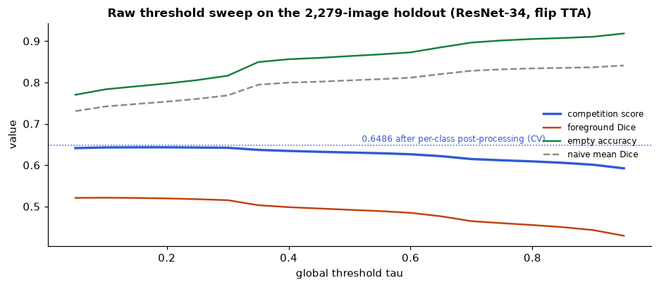
The model saves holdout probabilities as bytes from 0 to 255. The simplest rule is a global threshold \(\tau\): a pixel is defective when its probability is at least \(\tau\). The raw sweep over the whole 2,279-image holdout looks like this:
Threshold sweep explorer
Hold the pointer over the chart for exact values, and toggle the lines. Every point is computed from the saved holdout probabilities (val_probs.npy) and masks.
Raising the threshold removes weak, uncertain pixels. That helps empty accuracy (0.77 at tau 0.05, 0.92 at tau 0.95) but costs foreground Dice (0.52 down to 0.43). Naive mean Dice follows empty accuracy because 84% of its pairs are empty, so it prefers high thresholds. The official score weights foreground Dice at 70%, so it prefers low ones. This is the metric trade-off from lesson 3 playing out on real predictions.
Three rules for each class
A global threshold treats all classes alike, but they differ: defect_d blobs are big and low in contrast, while defect_a blobs are tiny. src/postproc.py therefore gives each class three parameters:
thr: the pixel probability threshold.comp_min: remove connected components smaller than this many pixels.area_min: if the surviving mask has fewer total pixels than this, predict nothing for the whole image and class.
def apply(prob, params):
    out = np.zeros(prob.shape, dtype=bool)
    for c, name in enumerate(CLASSES):
        p = params[name]
        b = (prob[c] >= round(p["thr"] * 255)).astype(np.uint8)
        n, labels, stats, _ = cv2.connectedComponentsWithStats(b, connectivity=8)
        keep = np.zeros(n, dtype=bool)
        keep[1:] = stats[1:, cv2.CC_STAT_AREA] >= p["comp_min"]
        m = keep[labels]
        if m.sum() >= p["area_min"]:
            out[c] = m
    return out
Post-processing on real validation images
Pick a holdout image and a class, then move the sliders. The probability map comes from the trained ResNet-34 model. Dice is computed against the true mask live. Press Use tuned values to load the project's parameters for that class.
Ground truth
Probability map (brighter means a higher probability)
Prediction after your rules
The demo stores each image at half resolution (64 × 400) to keep the page small. Pixel counts are scaled by 4 to full-resolution equivalents, and Dice is computed at half resolution, so values can differ slightly from the full-size evaluation.
Tuning without fooling yourself
The tuner is a plain grid search over 7 thresholds (0.05 to 0.5), 6 values of comp_min (0 to 400), and 8 values of area_min (0 to 4,000) for each class. That is 336 combinations per class. Because the score is a sum over pairs divided by fixed pair counts, each class's contribution can be maximised independently, which keeps the search cheap.
Any parameter tuned on the holdout will look good on the holdout. To measure honestly, src/evaluate.py uses 2-fold cross-validation: it shuffles the holdout into two halves, tunes on one half, and scores on the other, then swaps and averages.
| Setting | Score | Foreground Dice | Empty accuracy |
|---|---|---|---|
| Global tau 0.3 (raw) | 0.6420 | 0.5152 | 0.8163 |
| Tuned per class, 2-fold CV | 0.6486 | 0.5176 | 0.8659 |
| Tuned per class, in-sample | 0.6491 | 0.5184 | 0.8657 |
The gap between the cross-validated score (0.6486) and the in-sample score (0.6491) is only 0.0005, so the tuning isn't badly overfit to the holdout. The gain over the raw threshold is 0.0066. About 0.005 of it comes from empty accuracy rising by 0.05, and about 0.002 from foreground Dice.
The tuned parameters
The final parameters, tuned on the whole holdout, are saved in runs/r34_baseline/postproc.json:
| Class | thr | comp_min (px) | area_min (px) |
|---|
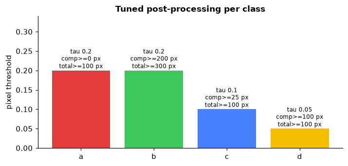
Notice that all thresholds are low, consistent with a metric that rewards recall. defect_d uses the lowest threshold (0.05) paired with a component filter of 100 pixels. A plausible reading is that the model is less confident on this class, so the tuner accepts weak pixels but discards small specks. defect_b, the rare class, has the strictest component filter (200 pixels) and a 300-pixel total minimum, which fits a rare class where false alarms are a risk.
See it as a video
This clip sweeps the global threshold from 0.05 to 0.95 and back on three real holdout images. The chart below the images shows the whole-holdout curves from the figure earlier, with a marker that follows the threshold.
Naive mean Dice rises as you increase the threshold from 0.05 to 0.95, but the competition score falls. Why?
- Naive Dice is dominated by empty pairs, which prefer quiet predictions, while the competition score weights foreground Dice at 70%.
- The competition score ignores empty pairs.
- Higher thresholds produce more false positives.
Higher thresholds make more empty pairs correct, which raises naive Dice. But they remove true defect pixels, which lowers foreground Dice and the weighted score.
The post-processing parameters come from tuning on the holdout. How does the project estimate the score on unseen data?
- It reports the in-sample score.
- It uses the test set.
- It tunes on half the holdout and scores on the other half, then swaps (2-fold CV).
The CV score is 0.6486 and the in-sample score is 0.6491. The CV number is the one the project reports.