Section 1 · Lesson 5
Training the model
The recipe is short: BCE plus Dice loss, light augmentation, AdamW with a one-cycle schedule, and a holdout score after every epoch.
- Which loss, optimiser, and schedule
src/train.pyuses. - What the augmentations do to an image and its mask.
- How to read the training curves, including the noisy parts.
The recipe
| Setting | Value in r34_baseline |
|---|---|
| Data | 9,114 training images, 2,279 holdout images (lesson 2) |
| Model | Unet with resnet34, ImageNet weights |
| Loss | BCE with logits + multilabel Dice (dice_w = 1.0) |
| Optimiser | AdamW, learning rate 3e-4, weight decay 1e-4 |
| Schedule | One-cycle, peak at 10% of the steps |
| Batch size and epochs | 16 and 10 |
| Device | Apple-silicon GPU (mps); 203 to 251 seconds per epoch |
The whole training loop is short enough to read in one go:
opt = torch.optim.AdamW(model.parameters(), lr=args.lr, weight_decay=1e-4)
steps = args.epochs * len(tr_dl)
sched = torch.optim.lr_scheduler.OneCycleLR(opt, max_lr=args.lr, total_steps=steps, pct_start=0.1)
bce = torch.nn.BCEWithLogitsLoss()
dice = pos_dice_loss if args.loss == "pos" else smp.losses.DiceLoss("multilabel", from_logits=True)

for img, msk in tr_dl:
    logits = model(img)
    loss = bce(logits, msk) + args.dice_w * dice(logits, msk)
    opt.zero_grad(set_to_none=True)
    loss.backward()
    opt.step()
    sched.step()
Loss
The loss adds two terms. Binary cross-entropy (BCE) looks at every pixel on its own and gives smooth gradients. Dice loss is \(1 - \mathrm{Dice}\) computed on the predicted probabilities, so it directly pushes up the overlap that the metric measures. It also copes with the fact that defect pixels are a tiny fraction of the image.
The project added a second option, --loss pos, for an experiment. It averages Dice only over pairs whose true mask is non-empty, so empty pairs don't pull the loss toward predicting nothing:
def pos_dice_loss(logits, targets):
    probs = logits.sigmoid()
    inter = (probs * targets).sum((-2, -1))
    denom = probs.sum((-2, -1)) + targets.sum((-2, -1))
    dice = (2 * inter + 1) / (denom + 1)
    pos = (targets.sum((-2, -1)) > 0).float()
    return ((1 - dice) * pos).sum() / pos.sum().clamp_min(1)
The r34_pos run used this loss with --oversample 2.0, which draws images containing defect_a or defect_b twice as often. The folder holds only its arguments file, and its log is empty, so this course can't report a result for it.
Augmentation
Augmentation shows the model slightly different versions of each image. The project applies these with the Albumentations library, to the image and the mask together:
A.Compose([
    A.HorizontalFlip(p=0.5),
    A.VerticalFlip(p=0.5),
    A.RandomBrightnessContrast(0.15, 0.15, p=0.5),
    A.ShiftScaleRotate(shift_limit=0.05, scale_limit=0.1, rotate_limit=0,
                       border_mode=0, p=0.3),
])
The mask must receive the same geometric change as the image, otherwise the labels no longer line up. Brightness and contrast change only the image.
Augmentation lab
Real training image with its defect_d mask. Change the controls, or press Random to draw one augmentation with the project's probabilities. The mask moves with the image.
Preview only: the browser draws brightness and contrast with its own filter, which is close to but not identical to the Albumentations version.
The learning-rate schedule
The one-cycle schedule starts at a low rate, ramps up to max_lr over the first 10% of the steps, and then decays smoothly toward zero. Warm-up protects the pretrained weights early on, and the long decay lets the model settle. PyTorch's defaults start at max_lr / 25 and end at that start value divided by 10,000.
One-cycle schedule
There are 569 optimiser steps per epoch (9,114 images, batch size 16, last partial batch dropped). The chart uses PyTorch's default cosine annealing with max_lr 3e-4.
Reading the curves
The training script prints one JSON line per epoch with the loss and the holdout score at four thresholds. Here are the real numbers for the baseline:
| Epoch | Train loss | Holdout score at 0.3 | Foreground Dice at 0.3 | Seconds |
|---|
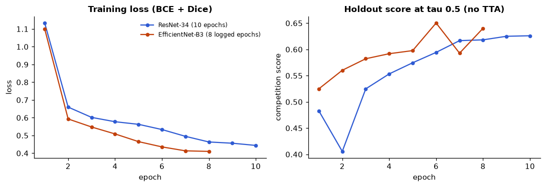
Compare the runs
Four observations from the files:
- Epoch 2 is worse than epoch 1. The holdout score at tau 0.3 drops from 0.4309 to 0.4141, and foreground Dice from 0.2825 to 0.1656. The learning rate peaks around the end of epoch 1, so a brief setback while it is highest is plausible. The model recovers by epoch 3.
- The score is still rising at epoch 10. The score at 0.3 goes 0.6186, 0.6205, 0.6271, 0.6284 over the last four epochs, so a longer run might help. The files don't test that.
- The EfficientNet-B3 curve is noisy. Its score at tau 0.5 reaches 0.6503 at epoch 6, falls to 0.5928 at epoch 7, and recovers to 0.6402 at epoch 8. A holdout with few images of the rare classes can make the score swing between epochs.
- Flip augmentation at test time helps. After the last epoch, averaging the model's predictions over the original and two flipped copies lifts the score at 0.3 from 0.6284 to 0.6420 (log line "TTA"). Lesson 7 explains this.
The Milestone 1 starter model, trained for 8 epochs, reports a final validation loss of 0.2785 and an assessment score of 0.5627 to 0.5677 across thresholds. It is a reference point, not a rival: its numbers come from a different script and loss.
Why does the training code apply the same flip to both the image and the mask?
- Flipping the mask makes the loss smaller.
- The mask pixels must stay aligned with the image pixels they label.
- Flips are only applied at test time.
If only the image flipped, the labelled pixels would point at the wrong place. Geometric augmentations must move the image and mask together.
The one-cycle schedule with pct_start=0.1 and 10 epochs reaches its peak learning rate roughly when?
- At the end of epoch 1
- At the end of epoch 5
- At the last step
10% of the steps is one epoch of ten. After the peak, the rate decays toward zero for the remaining nine epochs.