Section 2 · Lesson 7
Blend models and write the submission
Blend probabilities from different model families and turn them into the final submission file.
- Why averaging a multiclass and an ordinal model beats either alone.
- How the notebook trains on five folds and averages test predictions.
- How the final scores stack up, from 0.7520 to 0.7577.
- How to write and sanity-check
submission.csv.
Why blending works
Two models that make different mistakes can correct each other when you average their probabilities. Model quality isn't the only thing that matters: the ordinal LightGBM model scored only slightly higher than the multiclass one, but it added more to a CatBoost blend than another multiclass model did, because its errors differ.
The model experiments tested blends on the fold-0 holdout. Blend weights came from a 0.1-step grid that minimizes holdout log loss. The "cross-fitted weighted" column applies per-class weights fit on one half and scored on the other half.
| Blend | Argmax F1 | Log loss | Cross-fitted weighted F1 |
|---|---|---|---|
| CatBoost d8 + LightGBM (equal) | 0.7472 | 0.5805 | 0.7474 |
| CatBoost d8 + CatBoost d6 (equal) | 0.7456 | 0.5844 | 0.7459 |
| CatBoost d8 + ordinal LightGBM (equal) | 0.7502 | 0.5781 | 0.7498 |
| 0.3 CatBoost d8 + 0.3 CatBoost d6 + 0.2 ordinal + 0.2 ordinal (second seed) | 0.7516 | 0.5751 | 0.7519 |
Blends that include a mix of model families beat blends of near-identical models. Two CatBoost models averaged together gained less than a CatBoost plus an ordinal LightGBM.
Blend explorer on real holdout predictions
The three models are the saved fold-0 predictions of LightGBM multiclass, ordinal LightGBM, and CatBoost (15,000-row sample). Change the weights and watch the macro F1 and the log loss. Log loss is a steadier guide than macro F1, because it doesn't depend on a single argmax cut.
Which blend gains more, two CatBoost models with different depths or one CatBoost and one ordinal LightGBM?
- Two CatBoost models, because both are strong.
- CatBoost plus ordinal LightGBM (0.7502 against 0.7456), because the models make different errors.
- They gain the same.
Diversity matters more than strength. See the blend table in this lesson.
The final recipe
The final notebook is deliberately simpler than the experiments. It trains two LightGBM models per fold and leaves CatBoost out. Both use the same parameters: learning rate 0.05, 127 leaves, 80% feature and row subsampling, and early stopping after 100 rounds without improvement on the fold's validation set.
for i, (fit, val) in enumerate(folds):
    Xf, Xv = X_train.iloc[fit], X_train.iloc[val]
    p_val, p_test = fit_predict({**PARAMS, "objective": "multiclass", "num_class": K},
                                Xf, y[fit], Xv, y[val], X_test)
    oof["multiclass"][val] = p_val
    pred["multiclass"] += p_test / FOLDS            # average test predictions over folds
    # ... three binary models for the ordinal version, same pattern ...

blend_oof = (oof["multiclass"] + oof["ordinal"]) / 2
weights = tune_class_weights(blend_oof)
Every fold model also predicts the test set. The notebook averages those five test predictions, which acts like a five-model ensemble for each model type.
The scores
| Stage | 5-fold CV macro F1 |
|---|---|
| Multiclass LightGBM | 0.7520 |
| Ordinal LightGBM | 0.7547 |
| Blend (average) | 0.7559 |
Blend with class weights [1, 0.98, 1.15, 0.852] | 0.7577 |
The notebook's guide says that these CV scores understate the expected test score by about 0.004 (Lesson 6). The 0.7577 is also slightly optimistic, because the class weights are tuned on the same predictions that report the score. A cross-fitted check put the real gain from the weights at about +0.001.
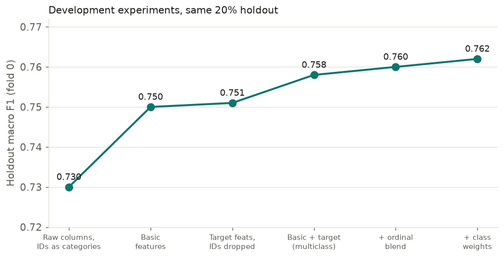
NOTEBOOK_GUIDE.md. The weighted blend (0.762) is tuned in-sample.build/04_videos.py).Write the submission
The last cell applies the class weights to the averaged test probabilities and writes the CSV with the columns ID and price_tier:
submission = pd.DataFrame({"ID": test["space_id"],
                           "price_tier": (blend_test * weights).argmax(1) + 1})
submission.to_csv("submission.csv", index=False)
Remember the + 1: the models use labels 0 to 3, and the competition wants 1 to 4. The following table shows the predicted tier counts for the 114,538 test listings, next to the training shares.
| Tier | Test predictions | Share of test | Share of train |
|---|---|---|---|
| 1 | 25,359 | 22.1% | 23.9% |
| 2 | 37,553 | 32.8% | 29.1% |
| 3 | 27,169 | 23.7% | 21.7% |
| 4 | 24,457 | 21.4% | 25.2% |
The test mix differs from the training mix, with more tier 2 and fewer tier 4. That might reflect a different test population, in which about a third of listings have unseen operators, or a model bias. The notebook can't tell you which, so treat it as a prompt to check, not as a verdict.
Check these before you submit. The file has one row per test listing and the columns ID and price_tier. The labels run from 1 to 4. The IDs come from the test file's space_id.
The notebook adds 1 to the argmax before it writes the submission. Why?
- The models predict 0 to 3, but the competition expects tiers 1 to 4.
- It breaks ties between classes.
- It applies the class weights.
The first cell converts price_tier to 0-based labels, and the last cell converts predictions back.